Big-O notation can appear intimidating. I get it. But believe it or not, once you get past the math jargon, it actually is very accessible. Trust me, take a deep breath, and dive in!

https://i.ytimg.com/vi/N5_sTEhnZKM/maxresdefault.jpg

Algorithms are simply step-by-step instructions for executing a specific task. We instruct the computer how to execute these steps in our source code, which is the code we write in our programming language of choice.
Big-O notation is a tool used by computer programmers to communicate how efficient an algorithm will run. Specifically, big-O notation will answer the question how long does it take an algorithm to run in the worse case scenario.
Why the worse case scenario? The actual running time of the algorithm will depend on how fast the computer is, what programming language is used, along with a handful of other factors. Theoretically, we want to be able to understand how our algorithm will work in general no matter what kind of computer or which programming language we are using. Determining the running time of the worse case scenario gives us a benchmark to compare the efficiency of one algorithm to another. Computer scientists also use big-θ notation to evaluate the average efficiency and big-Ω notation to evaluate the best possible performance of an algorithm, but it is more common to use big-O notation.
Practically, computer programmers want to be aware of how their code will perform under pressure. For example, if I am building a web application for myself and a handful of friends, I am not going to be concerned with how my web application performs with only a few users. However, the folks at Facebook need to be very concerned with how their code will run with millions of users interacting with their application at any given second. If any part of their code is inefficient, it will lead to poor performance and ultimately a very unhappy user. This is why we need to be mindful of worse case run time.
The nice thing about big-O notation is you just need to keep track of the part of the function that will grow fastest as the number of inputs (n) increase. This is the highest order term. By dropping the less significant terms and the constant coefficients, we can focus on the important part of an algorithm’s running time — its rate of growth — without getting stuck in details that complicate our understanding. Let’s get into concrete examples.
Searching Algorithms
O(1) Example: Constant Time Search
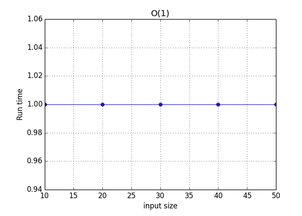
Suppose that an algorithm took a constant amount of time, regardless of the number of inputs (n). For example, if you were given an array that is already sorted in increasing order and you had to find the minimum value in the array, it would only take one step, since the minimum value must be at index 0.
big-o-1.rb
def minimum_value(array)
  return array[0]
end

minimum_value([0, 1, 2, 3, 4])
It doesn’t matter if the sorted array contains 5 elements or a million elements. This algorithm will perform the same no matter how many inputs.
https://mellowd.co.uk/ccie/?tag=big-o-notation
O(n) Example: Linear Search
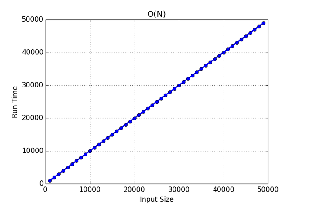
Linear search is a straightforward way to find a target value within an array. In the code below, we will return true if we find the target value in the array. In this example, we will need to loop through every single value in the array to determine if the current value matches the target value because our target value 4 is the last element of the array. For an array containing 5 elements (n = 5), that means it took us 5 steps to return true or false.
linear.rb
def linear_search(array, target)
  array.each do |i|
    if array[i] == target
      return true
    end
  end
  return false
end

linear_search([0,1,2,3,4], 4)
Linear search is O(n) because the number of inputs n is directly proportional to the number of steps we would have to take to execute our code in the worse case scenario.
https://mellowd.co.uk/ccie/?tag=big-o-notation
O(log n) Example: Binary Search
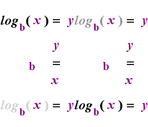
If this is where you see a logarithm and want run away, fight the urge! The logarithm function grows very slowly because logarithms are the inverse of exponentials, which grow very rapidly. An algorithm with exponential run time is horribly inefficient, while an algorithm with logarithmic run time is very efficient.
http://www.purplemath.com/modules/logs.htm
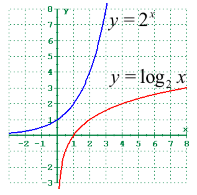
In the graph below the x-axis will represent n (the number of inputs) and the y-axis will represent the run time of the function as it relates to n. For the exponential function, we see the rate of growth doubles for each step. When n = 1, the rate of growth is 2. When n = 2, the rate of growth is 4. When n = 3, the rate of growth is 8.
https://people.richland.edu/james/lecture/m116/logs/logs.html
For the logarithmic function, we can see the rate of growth is cut in half at each step along the x-axis. When n = 2, the rate of growth is 1. When n = 3, the rate of growth is 1.5. When n = 4, the rate of growth is 2.
We will be using an algorithm called binary search, which will cut the rate of growth in half for each step of our code’s execution. This is why a logarithmic function is helpful to represent the relationship between n inputs and the run time of a function.
The binary search algorithm is fairly simple to implement and can dramatically improve the efficiency of our search for a value in an array. Let’s say we have a sorted array of a thousand elements (n = 1,000), and we are searching for a target value, and that target value is the very last element in the array. If we were to use linear search, we would have to take 1,000 steps to find our target value. Binary search will take at most 11 steps! Let’s find out why.

Video: CS50 2014 - Week 0, continued
With binary search, we will search through a sorted array for our target value. First we will check if the middle value in the array equals our target value. If the middle value equals the target value, we are done! If the middle value is less than the target value, we know that the target value must be somewhere in the second half of the array. That means the total number of inputs (n) is cut in half.
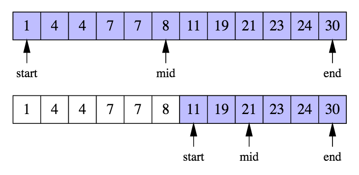
https://puzzle.ics.hut.fi/ICS-A1120/2015/notes/round-efficiency--binarysearch.html
If the middle value is greater than the target value, we know that the target value must be somewhere in the first half of the array. Again, that means the total number of inputs (n) is cut in half.
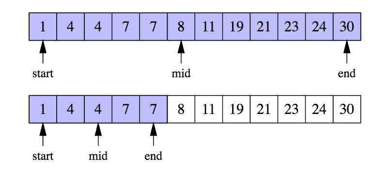
https://puzzle.ics.hut.fi/ICS-A1120/2015/notes/round-efficiency--binarysearch.html
We will keep cutting n in half after each failed guess until we finally reach the target value.
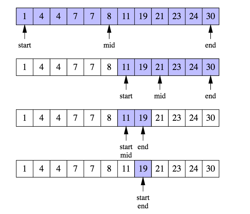
https://puzzle.ics.hut.fi/ICS-A1120/2015/notes/round-efficiency--binarysearch.html
We can execute this by reassigning the minimum or maximum index after each failed guess, which will cut the number of elements (n) we need to check in half.
binary_search.rb
def binary_search(array, target)
  min_index = 0
  max_index = (array.length) - 1

  while true
    return -1 if max_index < min_index

    guess_index = (min_index + max_index)/2

    if array[guess_index] == target
      return guess_index
    elsif array[guess_index] < target
      min_index = guess_index + 1
    elsif array[guess_index] > target
      max_index = guess_index - 1
    end
  end
end
As we can see in the graph below, the rate of the growth of a binary search function will be cut in half as the number of inputs (n)increase. If we have a small array, a linear search algorithm may outperform the binary search algorithm, but you can see that the binary search algorithm with O(log n) will outperform the linear algorithm as the the number of inputs (n) increase.
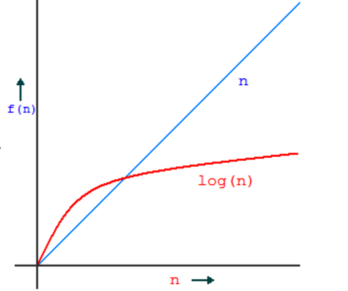
http://www.equestionanswers.com/c/c-binary-search.php
This is what we are concerned with when we talk about big-O notation. We are making very high-level generalizations about how an algorithm will perform as the number of inputs increase.
Sorting Algorithms
O(n log n) Example: Merge Sort
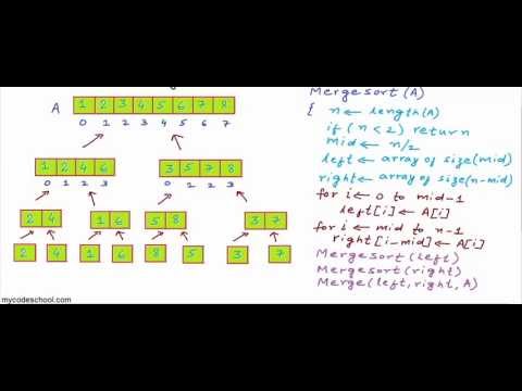
When you see O(n log n) you may still feel some aversion, but we have already examined O(n) with linear search and O(log n) with binary search. Merge sort is an example of a divide-and-conquer algorithm, which means we break a problem into subproblems that are similar to the original problem, recursively solve the subproblems, and finally combine the solutions to the subproblems to solve the original problem.
I would highly recommend watching this video below if you want to understand how merge sort works.
Video: Merge sort algorithm
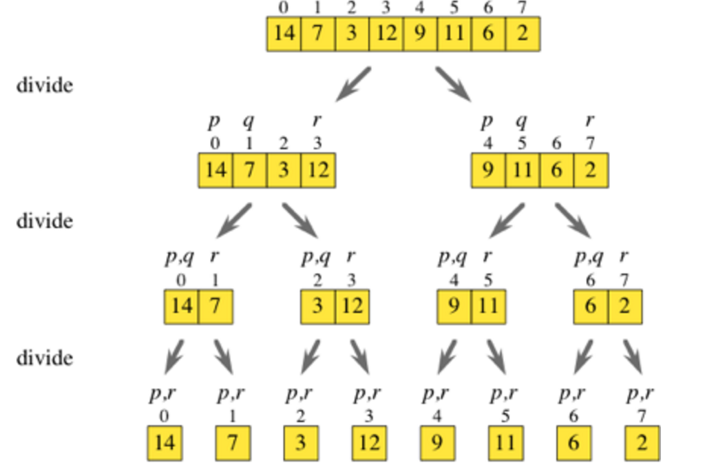
With the merge sort algorithm, we will continuously cut our array in half using recursion within the merge_sort function below. This is the part of the algorithm will run in O(log n) time because are continuously cutting the number of computations we need to execute per step in half, just like we did with binary search.
merge_sort.rb
def merge_sort(array)
  return array if array.length <= 1

  middle = array.length / 2
  left = merge_sort(array[0...middle])
  right = merge_sort(array[middle..-1])
  return merge(left, right)
end

def merge(left, right)
  result = []
  until left.empty? || right.empty?
    result << (left.first <= right.first ? left.shift : right.shift)
  end
  return result + left + right
end
The division part of our divide-and-conquer algorithm is shown in the diagram below:
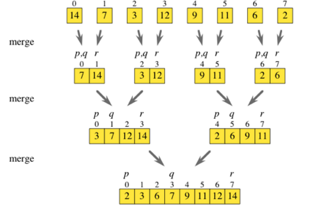
Once we reach the base case, we can pause and examine our two subproblems, which in merge sort are two separate arrays that need to be merged. The purpose of the merge function in the code above is to create a sorted array from our two unsorted subarrays, as demonstrated in the diagram below. The function merge will take O(n) time because we only need to check each element once in order to merge the two unsorted arrays into one sorted array.
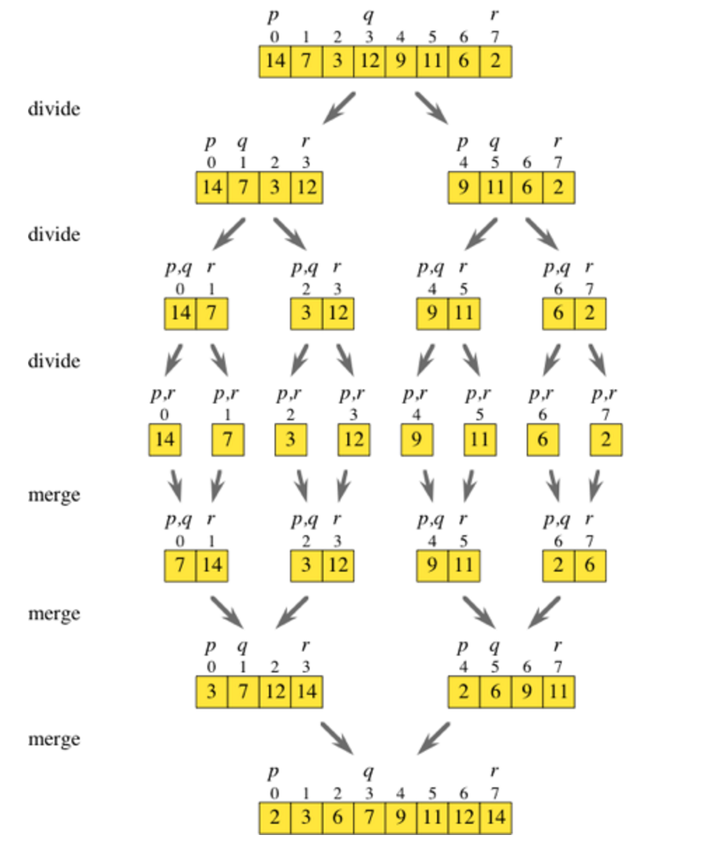
Overall, our algorithm will run O(n log n) or more explicitly O(n * log(n)) in order to execute total divide-and-conquer algorithm.
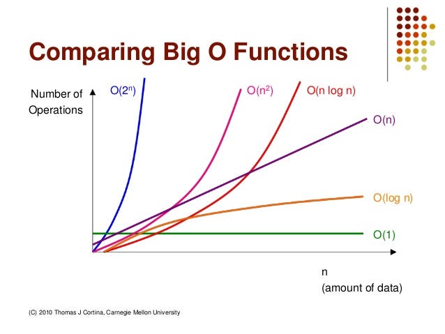
While O(n log n) is not the most efficient algorithm, it is still much better than the last one we are going to look at, O(n²).
O(n²) Example: Selection Sort
Let’s say we have an unsorted array = [22, 11, 7, 88, 9] with n = 5 elements. How can we create an algorithm that will sort the array from the smallest to largest and will output the sorted array =[7, 9, 11, 22, 88]? We will use selection sort to select the smallest value in the array and swap it with the current index. Our input array is:
unsorted array = [22, 11, 7, 88, 9]
This is the most intuitive yet least efficient approach. Let’s look at the element at index 0, 22. This will the be the current minimum value in the array. We will then loop through the rest of the array and determine if there is a number smaller than 22. Is 11 < 22? Yes, so 11 is our new minimum value. Is 7 < 11? 7 is smaller than 11, so this is our new minimum. Is 88 < 7? No. Is 9 < 7? No. Now we will swap the zero index value with the minimum value, at after this step our array will be:
unsorted array = [7, 11, 22, 88, 9]
At this point we know that 7 is the smallest value in our array, so we no longer need to check the zero index value in our array. We will now set our minimum value to 11. We will loop through the remaining subarray and determine the minimum value. Is 11 < 22. Yes. Is 11 < 88. Yes. Is 11 < 9? No, so our new minimum is 9. We have loop through the rest of the elements in the array and determine the minimum value is 9, so we swap 11 and 9.
unsorted array = [7, 9, 22, 88, 11]
We know that our subarray [7, 9] is sorted, so we will now set our minimum value to 22. Is 22 < 88? Yes. Is 22 < 11? No, so 11 is our new minimum value. We will swap the current index 22 with the new minimum 11 and our array is now:
unsorted array = [7, 9, 11, 88, 22]
The subarray [7, 9, 11] is sorted, so we will start with setting our minimum value to 88. Is 88 < 22? No, so our new minimum value is 22, and we will swap 88 and 22 and return:
sorted array = [7, 9, 11, 22, 88]
This is what our algorithm will look like, using two helper functions (swap and index_of_minimum) to execute the selection_sort function.
selection_sort.rb
# swap the location of two items in the array
def swap(array, first_index, second_index)
  temp = array[first_index]
  array[first_index] = array[second_index]
  array[second_index] = temp
  return array
end

# find index of minimum value in the subarray (from the start_index to the end)
def index_of_minimum(array, start_index)
  min_value = array[start_index]
  min_index = start_index

  for i in (start_index+1)..(array.length-1) do
    if min_value > array[i]
      min_value = array[i]
      min_index = i
    end
  end
  return min_index
end

# selection sort repeatedly selects the next-smallest element and swaps it into place
def selection_sort(array)
  array.each_with_index do |start_value, start_index|
    min_index = index_of_minimum(array, start_index)
    swap(array, start_index, min_index)
  end
end
The swap helper function will take constant time or O(1). The selection sort algorithm requires two for loops, one in the main selection_sort function and one in the index_of_minimum helper function. A good rule of thumb is any function that requires looping through an array will take O(n) because in the worse case scenario we will have to iterate through every element (n) in the array. In the worse case scenario when looping within a loop, we would have to perform n actions per each n elements in the array, or in this case 5 actions * 5 elements. Therefore, the worse case running time of selection sort will be O(n²).
I hope this helps a little big in demystifying big-O notation. Just keep exposing yourself to more and more algorithms and soon these concepts will settle in and make sense. Here is a cheatsheet to help you along the way. Be patient and have fun with it!